This article is a comprehensive guide to system identification — the process of building mathematical models of dynamical systems from measured input-output data. It covers the fundamental concepts and workflow of system identification, classical parametric methods, subspace identification, kernel-based regularized approaches, identification for periodically time-varying and multirate systems, polytopic uncertainty modeling, and the relationship between model-based identification and data-driven control design. Links to detailed articles, research papers, videos, and MATLAB codes are provided throughout.

A distinguishing feature of this guide is the coverage of cyclic reformulation, an approach developed in the author's research that transforms periodically time-varying and multirate identification problems into standard LTI identification problems. This enables the use of well-established subspace methods for systems that have traditionally required specialized algorithms.

Author: Hiroshi Okajima, Associate Professor, Kumamoto University, Japan — 20 years of control engineering research

Why System Identification Matters
What is System Identification?
Classical Parametric Methods
Subspace Identification Methods
Kernel-Based and Regularized Identification
Identification for Periodically Time-Varying Systems
Identification Under Multirate Sensing
Polytopic Uncertainty Modeling via Cyclic Reformulation
Other Identification Approaches
Beyond Identification: Data-Driven Control Design
After Identification: What's Next?
Connections to Related Topics
- Supporting Topics
- Cross-Cluster Links
Key References
Related Articles and Videos
Papers by the Author
- MATLAB Code
SystemIdentification #SubspaceIdentification #MultiRateSystems #CyclicReformulation #ControlEngineering #MATLAB #DataDrivenControl #StateSpaceModel #ParameterEstimation #SensorFusion #PolytopicUncertainty #RobustControl

Why System Identification Matters

In model-based control engineering, the quality of the controller depends directly on the quality of the plant model. Obtaining an accurate mathematical model is therefore the essential first step in any control design workflow.

There are two fundamental approaches to modeling. The first is first-principles modeling, where the equations of motion, circuit equations, or thermodynamic laws are used to derive the model analytically. The second is system identification, where the model is constructed from measured input-output data using statistical or algebraic algorithms.

System identification is indispensable when:

The physical laws governing the plant are too complex or partially unknown — for example, in biological systems, chemical processes, or flexible structures with uncertain parameters.
A quick and accurate model is needed for controller tuning — rather than spending weeks deriving first-principles equations, a few minutes of input-output data can produce an accurate model.
The plant operates in a multirate sensing environment — different sensors provide data at different sampling rates, and the model must be identified from such heterogeneous data.
Online adaptation is required — the plant parameters change over time, and the model must be updated continuously. Recursive identification methods (discussed in "Other Identification Approaches" below) address this scenario.

Once a model is identified, it enables a wide range of model-based design tasks: state observer design, Kalman filtering, model predictive control (MPC), robust control using the Model Error Compensator (MEC), and more.

This article serves as a hub connecting the various aspects of system identification theory and practice. Each section below provides an overview with links to detailed articles for deeper study.

System Identification Sequence — System Identification

What is System Identification?

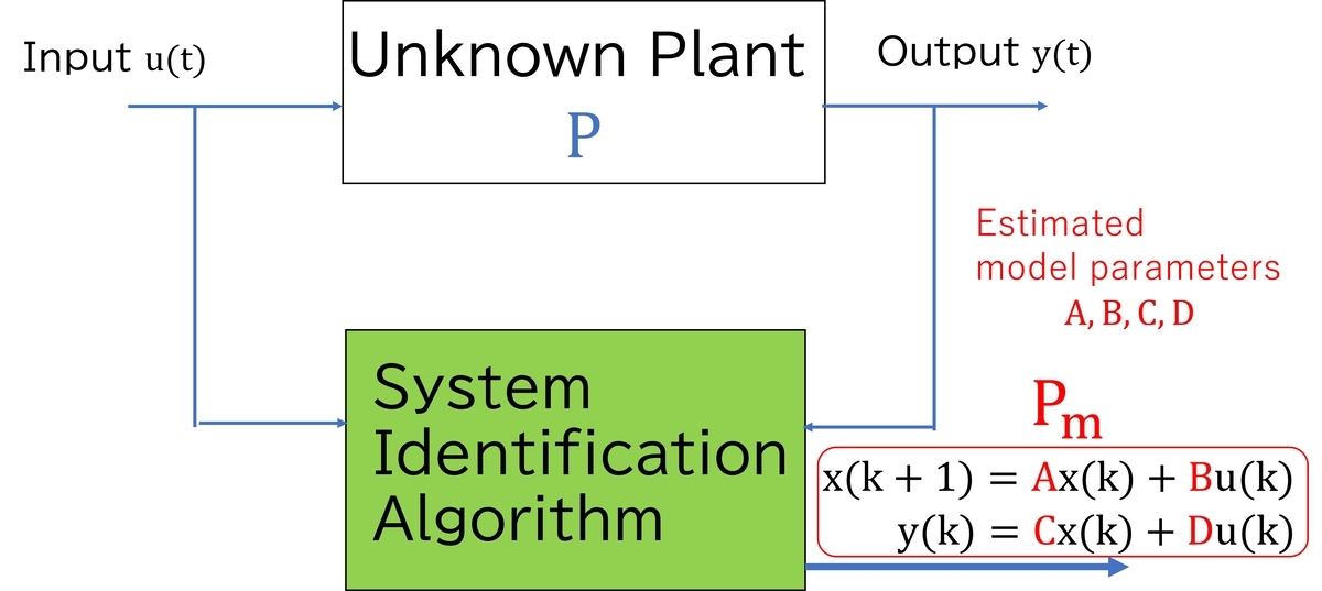
System identification is the process of estimating a mathematical model of a dynamical system from observed input-output data. The standard treatment is given in the textbook by Ljung [L1] and the monograph by Söderström and Stoica [L2], which remain the primary references in the field. The general workflow consists of four steps:

Step 1: Data acquisition — Apply an input signal $u(k)$ to the plant and record the output signal $y(k)$ . The input should be sufficiently rich in frequency content to ensure that the model parameters are uniquely identifiable. This requirement is formalized as the persistent excitation condition: the input signal must have enough spectral content to excite all modes of the system. In practice, random signals (e.g., pseudo-random binary sequences) or swept sinusoids are commonly used to achieve this. Persistent excitation is a necessary condition for parameter identifiability in both parametric methods [L1] and subspace methods [L3].

Step 2: Model structure selection — Choose a model class. Common choices include transfer function models (ARX, ARMAX, Output-Error, Box-Jenkins), state-space models, and nonparametric representations such as impulse responses or frequency responses.

Step 3: Parameter estimation — Apply an identification algorithm to estimate the model parameters $\theta$ from the data. Methods range from least-squares and prediction error methods to subspace identification and regularized estimation.

Step 4: Model validation — Assess the quality of the identified model using techniques such as cross-validation, residual analysis, or comparison of predicted and measured outputs on a separate validation dataset. A common quantitative metric is the FIT value, defined as:

$\displaystyle \mathrm{FIT} = 100 \times \left(1 - \frac{\|y - \hat{y}\|}{\|y - \bar{y}\|}\right) \quad [\%$ ]

where $y$ is the measured output, $\hat{y}$ is the model-predicted output, and $\bar{y}$ is the mean of the measured output. A FIT of 100% indicates perfect prediction, while a FIT of 0% means the model performs no better than the sample mean. This metric is used in MATLAB's compare function and throughout the identification literature. It is also used in the numerical examples of Sections 5–7 of this article.

In discrete-time system identification, the goal is typically to obtain a state-space model:

$\displaystyle x(k+1) = Ax(k) + Bu(k)$

$\displaystyle y(k) = Cx(k) + Du(k)$

or an equivalent transfer function representation. Once a discrete-time model is obtained, it can be converted to a continuous-time model if needed.

For an introduction to system identification with MATLAB simulation examples, see the blog article: System Identification: Obtaining Dynamical Model

Classical Parametric Methods

Classical parametric identification methods assume a specific model structure with unknown parameters and estimate these parameters using prediction error minimization or least-squares methods. This framework is systematically developed in Ljung [L1] and Söderström & Stoica [L2]. The most widely used model structures are:

ARX (Auto-Regressive with eXogenous input) — The simplest structure, where the output is a linear combination of past outputs, past inputs, and a white noise term. The model is:

$\displaystyle A(q^{-1})y(k) = B(q^{-1})u(k) + e(k)$

where $A(q^{-1}) = 1 + a_{1}q^{-1} + \cdots + a_{n_a}q^{-n_a}$ and $B(q^{-1}) = b_{1}q^{-1} + \cdots + b_{n_b}q^{-n_b}$ are polynomials in the backward shift operator $q^{-1}$ (i.e., $q^{-1}y(k) = y(k-1)$ ), and $e(k)$ is white noise. The parameters can be estimated by ordinary least squares, making ARX computationally efficient.

ARMAX (Auto-Regressive Moving Average with eXogenous input) — Extends ARX by adding a moving average model for the noise:

$\displaystyle A(q^{-1})y(k) = B(q^{-1})u(k) + C(q^{-1})e(k)$

This provides more flexibility in modeling the noise characteristics.

Output-Error (OE) — Models the plant dynamics directly without noise filtering:

$\displaystyle y(k) = \frac{B(q^{-1})}{F(q^{-1})}u(k) + e(k)$

Box-Jenkins (BJ) — The most general structure, which separately models the plant dynamics and the noise dynamics:

$\displaystyle y(k) = \frac{B(q^{-1})}{F(q^{-1})}u(k) + \frac{C(q^{-1})}{D(q^{-1})}e(k)$

The model structures form a hierarchy: ARX is the simplest, while Box-Jenkins is the most general. ARMAX and OE are intermediate structures. The choice among these structures involves a trade-off between model flexibility and estimation complexity. MATLAB's System Identification Toolbox provides functions such as arx, armax, oe, and bj for these methods.

A key challenge in parametric methods is model order selection — determining the appropriate polynomial orders. Common approaches include information criteria (AIC, BIC), cross-validation, and residual analysis.

The Prediction Error Method (PEM) is the unifying estimation framework behind ARMAX, OE, and Box-Jenkins. PEM minimizes the sum of squared one-step-ahead prediction errors $\varepsilon(k, \theta) = y(k) - \hat{y}(k|k-1,\theta)$ over the parameter vector $\theta$ , typically via Gauss-Newton or Levenberg-Marquardt iteration. The ARX model is the special case where PEM reduces to ordinary least squares [L1].

For the detailed treatment of classical parametric methods and the prediction error method, see: Classical Parametric System Identification: ARX, ARMAX, and the Prediction Error Method

Subspace Identification Methods

Subspace identification methods provide a fundamentally different approach to system identification. Instead of estimating polynomial coefficients, they directly estimate the state-space matrices $A, B, C, D$ from input-output data using linear algebra techniques — specifically, singular value decomposition (SVD) of structured data matrices. The standard references for this approach are the books by Katayama [L3] and Verhaegen & Verdult [L4], and the survey by Qin [L5].

The core idea is to construct block Hankel matrices from the input-output data and extract the extended observability matrix and state sequences through SVD. A block Hankel matrix is a structured matrix formed by arranging the data in overlapping blocks — for example, the output block Hankel matrix with $i$ block rows and $j$ columns is:

$\displaystyle Y_{0|i-1} = \begin{pmatrix} y(0) & y(1) & \cdots & y(j-1) \cr y(1) & y(2) & \cdots & y(j) \cr \vdots & \vdots & \ddots & \vdots \cr y(i-1) & y(i) & \cdots & y(i+j-2) \end{pmatrix}$

The key observation is that the column space of the output block Hankel matrix (after removing the input effect) coincides with the column space of the extended observability matrix:

$\displaystyle \mathcal{O}_i = \begin{pmatrix} C \cr CA \cr CA^2 \cr \vdots \cr CA^{i-1} \end{pmatrix}$

Since the rank of $\mathcal{O}_{i}$ equals the system order $n$ (assuming observability), the singular values of the processed data matrix provide a natural indicator of model order: the number of significant singular values corresponds to $n$ .

The three major subspace identification algorithms are:

N4SID (Numerical algorithms for Subspace State Space System IDentification) — Uses oblique projections to estimate the state sequence and then determines the system matrices by least squares [L6].

MOESP (Multivariable Output-Error State Space) — Uses instrumental variable techniques and orthogonal projections [L7].

CVA (Canonical Variate Analysis) — Uses canonical correlations between past and future data to determine the system order and state estimates. The statistical foundations of CVA for state-space identification were developed by Larimore [L8].

The advantages of subspace methods over classical parametric methods include:

No iterative optimization — the computation relies on SVD and least squares, avoiding local minima problems.
Natural handling of multivariable systems — MIMO systems are treated as naturally as SISO systems.
Direct state-space output — no intermediate polynomial representation is needed.
Automatic model order determination — the singular values of the data matrices provide a natural indicator of system order (as described above).

MATLAB provides the n4sid function in the System Identification Toolbox. Subspace identification is also the foundation for the author's research on periodically time-varying and multirate system identification (see Sections 5–7 below), where the cycled system is identified using standard subspace methods as a key algorithmic step.

For the detailed tutorial on N4SID, MOESP, and CVA, see: Subspace System Identification: A Tutorial on N4SID, MOESP, and CVA with MATLAB

Kernel-Based and Regularized Identification

A more recent paradigm in system identification is kernel-based (regularized) identification, which avoids the model order selection problem by estimating impulse responses directly in a regularized framework [L9].

Instead of assuming a finite-dimensional parametric model, the impulse response $g(k)$ is estimated as a function in a reproducing kernel Hilbert space (RKHS). The estimation problem becomes:

$\displaystyle \hat{g} = \arg\min_{g} \sum_{k} \bigl(y(k) - \hat{y}(k)\bigr)^2 + \lambda \|g\|_{\mathcal{H}}^2$

where $\lambda > 0$ is a regularization parameter and $|\cdot|_{\mathcal{H}}$ is the RKHS norm induced by the kernel. The kernel encodes prior knowledge about the impulse response — for example, the stable spline kernel enforces exponential decay, which is appropriate for stable LTI systems.

Key features of kernel-based identification:

No model order selection — the regularization automatically controls model complexity.
Bayesian interpretation — the regularized estimate corresponds to the maximum a posteriori (MAP) estimate under a Gaussian process prior.
Hyperparameter tuning — the kernel parameters and regularization strength are estimated by marginal likelihood maximization (empirical Bayes).
Smooth interpolation — the estimated impulse response is smooth and less sensitive to noise than parametric estimates of comparable accuracy.

MATLAB's impulseest function supports regularized impulse response estimation. The theoretical foundations are covered in the survey by Pillonetto, Dinuzzo, Chen, De Nicolao, and Ljung [L9].

Compared to classical parametric methods and subspace identification, kernel-based methods represent a complementary approach: parametric methods are best when the model structure is known, subspace methods excel for moderate-dimensional state-space models, and kernel methods shine when the model order is uncertain or high.

Identification for Periodically Time-Varying Systems

Many control systems are inherently periodically time-varying (LPTV) — their dynamics change cyclically over time. Examples include systems with periodic scheduling, sampled-data systems, and systems with periodic disturbances. The theoretical foundation for cyclic reformulation of discrete-time periodic systems was established by Bittanti and Colaneri [L10, L11].

An LPTV system has the form:

$\displaystyle x(k+1) = A_k x(k) + B_k u(k)$

$\displaystyle y(k) = C_k x(k) + D_k u(k)$

where $A_{k} = A_{k+M}$ , $B_{k} = B_{k+M}$ , $C_{k} = C_{k+M}$ , $D_{k} = D_{k+M}$ for some period $M$ . The identification problem is to estimate the $M$ sets of matrices ${A_{k}, B_{k}, C_{k}, D_{k}}_{k=0}^{M-1}$ .

The cyclic reformulation approach transforms the LPTV system into an equivalent higher-dimensional LTI system by constructing cycled signals. The key idea is to "spread" the original scalar signal across an $M$ -dimensional vector: at each time step, the original sample is placed in the vector position corresponding to $k \bmod M$ , while the remaining positions are filled with zeros. The resulting cycled input $\check{u}(k) \in \mathbb{R}^{Mm}$ and cycled output $\check{y}(k) \in \mathbb{R}^{Ml}$ form the input-output data for an equivalent LTI system with cyclic structure in its state-space matrices.

The resulting cycled system:

$\displaystyle \check{x}(k+1) = \check{A}\,\check{x}(k) + \check{B}\,\check{u}(k)$

$\displaystyle \check{y}(k) = \check{C}\,\check{x}(k) + \check{D}\,\check{u}(k)$

is an LTI system with cyclic structure in its matrices. This LTI system can be identified using standard subspace identification methods (e.g., N4SID). After identification, a state coordinate transformation is applied to recover the cyclic structure, and the original LPTV parameters are extracted from the structured matrices. The mathematical details of the cycled signal construction, the cyclic matrix structure, and the state coordinate transformation are given in the detailed article linked below.

This approach is particularly powerful because:

It works with arbitrary (non-periodic) input signals — no special input signal design is required, as long as the persistent excitation condition is satisfied for the cycled system.
The computational effort is comparable to standard LTI identification.
The identified model directly provides the periodic matrices needed for LPTV controller and observer design.

For the full theoretical development including the precise definition of cycled signals and the state coordinate transformation, see the blog article: Cyclic Reformulation-Based System Identification for Periodically Time-Varying Systems

Paper: H. Okajima, Y. Fujimoto, H. Oku and H. Kondo, Cyclic Reformulation-Based System Identification for Periodically Time-Varying Systems, IEEE Access (2025)

Identification Under Multirate Sensing

In modern control systems, multiple sensors with different sampling rates are commonly used. For example, in mobile robot control, cameras, LiDAR, IMUs, and wheel encoders all operate at different rates. In industrial process control, temperature sensors, pressure sensors, and flow meters may have very different observation periods.

The multirate identification problem is a special case of the LPTV identification problem described above. The underlying plant is a standard discrete-time LTI system:

$\displaystyle x(k+1) = Ax(k) + Bu(k)$

$\displaystyle y(k) = Cx(k) + Du(k)$

but the outputs are observed through a periodically time-varying diagonal matrix $V_{k}$ :

$\displaystyle y_{\mathrm{obs}}(k) = V_k C x(k) + V_k D u(k)$

where $V_{k} = \mathrm{diag}\lbrack v_{1}(k), \ldots, v_{l}(k) \rbrack$ , and $v_{i}(k) = 1$ when sensor $i$ is active (i.e., $k$ is a multiple of $M_{i}$ ) and $v_{i}(k) = 0$ otherwise. The frame period is $M = \mathrm{lcm}(M_{1}, \ldots, M_{l})$ .

A key structural insight is that in the multirate case, the plant itself is time-invariant — only the observation structure is periodic. This means the cyclic reformulation matrices $\check{A}$ and $\check{B}$ have identical blocks at every position, while the periodic structure appears only in $\check{C}$ and $\check{D}$ through the observation matrices $V_{k}$ . This leads to simpler controllability and observability conditions compared to the general LPTV case.

The identification algorithm consists of four steps:

Determine the frame period $M$ and construct cycled signals $\check{u}(k)$ and $\check{y}(k)$ from the measured data.
Apply a standard subspace identification method (e.g., N4SID) to the cycled signals to obtain an identified model.
Apply the state coordinate transformation to recover the cyclic reformulation structure.
Extract the time-invariant matrices $A, B, C, D$ from the structured cyclic matrices.

The algorithm works with arbitrary (non-periodic) inputs and achieves identification accuracy comparable to the single-rate case. Numerical examples demonstrate that the identified transfer functions match the true transfer functions to machine precision.

For the detailed algorithm and numerical results, see the blog article: System Identification Under Multirate Sensing Environments

Paper: H. Okajima, R. Furukawa and N. Matsunaga, System Identification Under Multirate Sensing Environments, Journal of Robotics and Mechatronics, Vol. 37, No. 5, pp. 1102–1112 (2025) (Open Access)

Code: Code Ocean

Polytopic Uncertainty Modeling via Cyclic Reformulation

A natural next step after system identification is to quantify model uncertainty for robust control design. Matrix polytope representation is the standard framework for this purpose: the system matrices are expressed as a convex combination of vertex matrices ${(A_{i}, B_{i}, C_{i}, D_{i})}_{i=0}^{N-1}$ , enabling the application of LMI-based robust control synthesis [L12].

Problem: Existing methods for polytopic model construction typically require multiple identification experiments or a priori assumptions about the uncertainty structure — both of which are costly and restrictive in practice.

Proposed approach: An algorithm that applies cyclic reformulation with period $N$ to a linear time-invariant system and uses the noise-induced parameter variations among the resulting $N$ parameter sets as polytope vertices. The underlying idea is:

Noise-free case: All $N$ parameter sets would be identical, reflecting the time-invariant nature of the true system.
Noisy case: The $N$ parameter sets exhibit variations around the true values due to process and observation noise. These variations are used as polytope vertices, and the optimal vertex weights are determined by optimization.

It should be noted that the theoretical justification for why noise-induced variations yield a valid polytopic uncertainty model (in the sense of guaranteeing that the true system lies within the polytope) remains an open question. The current paper provides empirical evidence that this approach improves prediction accuracy, but a rigorous theoretical guarantee is a subject for future work.

The optimal vertex weights $\lambda^{\ast}$ are found by Particle Swarm Optimization (PSO) to minimize a validation error. Numerical results on a 3rd-order SISO plant demonstrate consistent FIT improvement of 0.17–2.42 percentage points over conventional single-model identification across all tested noise conditions.

The period $N$ is a designer-selectable parameter: small $N \in {2,3,4}$ yields stable, low-error estimates; large $N$ increases computational burden as $O((Nn)^{3})$ and risks estimation degradation when data is insufficient. A practical guideline is that sufficient data length $N_{\mathrm{data}} > 10(Nn)^{2}$ is required for reliable polytope construction.

Paper (under review): H. Okajima, S. Shirahama, T. Hayashi and N. Matsunaga, "From Noise to Knowledge: System Identification with Systematic Polytope Construction via Cyclic Reformulation", IEEE Access (under review)

Other Identification Approaches

Beyond the methods described above, several other identification paradigms address specific application needs.

Frequency Domain Identification

Frequency domain methods estimate the frequency response (Bode plot) of the system directly from input-output data, using spectral analysis or frequency-domain transfer function fitting. These methods are natural when the system is excited by sinusoidal or periodic signals and are widely used in mechanical and structural engineering for modal analysis.

Recursive and Online Identification

Recursive identification methods such as Recursive Least Squares (RLS) and its variants update the model parameters incrementally as new data arrives, without storing and reprocessing the entire dataset. This is essential for adaptive control, where the model must track slowly varying plant parameters in real time — the "online adaptation" scenario mentioned in the introduction. By continuously updating the model, recursive methods enable the controller to maintain performance even when the plant characteristics change over the system's lifetime.

Closed-Loop Identification

When identification must be performed while the plant operates under feedback control (for safety or operational reasons), special techniques are required because the feedback creates correlations between the input and the noise. Methods include direct identification with high-order noise models, indirect identification using the known controller, and joint input-output approaches.

Machine Learning and Neural Network-Based Identification

Recent advances in machine learning have introduced new tools for system identification: NARX neural networks, recurrent neural networks (RNNs), physics-informed neural networks (PINNs), and deep state-space models. These methods can capture complex nonlinear dynamics but typically require large datasets and careful regularization. They offer a complementary perspective to classical model-based identification, particularly for systems where first-principles structure is difficult to formalize.

Beyond Identification: Data-Driven Control Design

An alternative to the "identify a model, then design a controller" paradigm is data-driven control design, where the controller parameters are tuned directly from input-output data without explicitly identifying a plant model. Key methods include:

VRFT (Virtual Reference Feedback Tuning) — A one-shot, offline method that computes a virtual reference signal from measured data and solves a least-squares problem to determine the controller parameters that best match a desired closed-loop transfer function.

FRIT (Fictitious Reference Iterative Tuning) — A related method developed in Japan that uses a fictitious reference signal concept for offline controller tuning from a single batch of closed-loop data.

IFT (Iterative Feedback Tuning) — An iterative method that performs gradient descent on a cost function evaluated directly from closed-loop experiments, without requiring a plant model.

Willems' Fundamental Lemma and Data-Driven Predictive Control — A framework based on the result by Willems, Rapisarda, Markovsky, and De Moor [L13] showing that all trajectories of an LTI system can be represented as linear combinations of a single, sufficiently exciting trajectory. This enables data-driven formulations of model predictive control (MPC) without explicit model identification.

These data-driven methods and the identification-based approach are not mutually exclusive — they represent complementary paradigms for control design. The identification-based approach combined with the Model Error Compensator (MEC) offers a different trade-off: the existing controller remains unchanged, and robustness is achieved by an add-on compensator. For a detailed comparison of these approaches, see the MEC hub article.

After Identification: What's Next?

An identified model enables a wide range of downstream control design tasks:

State observer and state estimation — The identified state-space model $(A, B, C, D)$ provides the plant model required for Luenberger observer design, Kalman filter design, and H∞ filter design. In multirate sensing environments, the identified multirate model (Section 6) directly feeds into the Multi-Rate Observer and the Multi-Rate Kalman Filter design.

See: State Observer and State Estimation: A Comprehensive Guide

Robust control with MEC — Since the identified model inevitably contains errors, the Model Error Compensator (MEC) can be combined with any existing controller to compensate for model inaccuracies without modifying the controller itself.

State feedback control design — The identified state-space model $(A, B, C, D)$ can be used directly for state feedback controller design using pole placement or LQR (Linear Quadratic Regulator). When only partial outputs are available, the identified model also enables observer-based feedback design via the separation principle.

See: State Feedback Control and State-Space Design: A Comprehensive Guide

Robust control with polytopic uncertainty — The polytopic uncertainty model (Section 7) constructed from cyclic reformulation can be used directly in LMI-based robust control synthesis [L12], gain-scheduled control, and robust filtering design.

Model Predictive Control (MPC) — MPC uses the identified model to predict future outputs and optimize the control input over a receding horizon. When combined with MEC, MPC gains robustness against model errors without the complexity of robust MPC formulations.

Model validation — After identification, the model should be validated on a separate dataset not used for estimation. Key validation techniques include comparing the simulated output with measured data (using the FIT metric defined in the "What is System Identification?" section above), analyzing the residuals (which should be white noise if the model is adequate), and testing the model's ability to predict multi-step-ahead outputs.

Supporting Topics

The following foundational topics support the theory and practice of system identification:

Controllability and Observability — Controllability ensures that the input can excite all modes of the system, while observability ensures that all modes are reflected in the output. Both are prerequisites for successful identification.
Discretization of Continuous-Time Control Systems — Connects continuous-time models obtained from first principles with the discrete-time models obtained from system identification.
Stability of State Equations — Stability analysis of the identified model is essential for ensuring that the identified system is physically meaningful.
Linear Matrix Inequalities (LMIs) and Controller Design — LMI tools are used both in the subsequent control and observer design based on the identified model, and in polytopic robust control synthesis.

Cross-Cluster Links

Observer Cluster: The identified model enables state observer and Kalman filter design. The multirate identification result (Section 6) is the prerequisite for the Multi-Rate Observer and Multi-Rate Kalman Filter.
MEC Cluster: The Model Error Compensator compensates for errors in the identified model without changing the existing controller.
State Feedback Cluster: The identified state-space model is used for state feedback control design — pole placement, LQR, and observer-based feedback via the separation principle.

Key References

The following texts are the primary references for system identification theory and practice:

[L1] L. Ljung, System Identification: Theory for the User, 2nd ed., PTR Prentice Hall, 1999.

[L2] T. Söderström and P. Stoica, System Identification, Prentice Hall, 1989.

[L3] T. Katayama, Subspace Methods for System Identification, Springer, Communications and Control Engineering Series, 2005.

[L4] M. Verhaegen and V. Verdult, Filtering and System Identification: A Least Squares Approach, Cambridge University Press, 2007.

[L5] S. J. Qin, "An overview of subspace identification," Computers & Chemical Engineering, vol. 30, no. 10–12, pp. 1502–1513, 2006.

[L6] P. V. Overschee and B. D. Moor, "N4SID: Subspace algorithms for the identification of combined deterministic-stochastic systems," Automatica, vol. 30, no. 1, pp. 75–93, 1994.

[L7] M. Verhaegen and P. Dewilde, "Subspace model identification Part 1: The output-error state-space model identification class of algorithms," International Journal of Control, vol. 56, no. 5, pp. 1187–1210, 1992.

[L8] W. E. Larimore, "Canonical variate analysis in identification, filtering, and adaptive control," Proceedings of the 29th IEEE Conference on Decision and Control, pp. 596–604, 1990.

[L9] G. Pillonetto, F. Dinuzzo, T. Chen, G. De Nicolao, and L. Ljung, "Kernel methods in system identification, machine learning and function estimation: A survey," Automatica, vol. 50, no. 3, pp. 657–682, 2014.

[L10] S. Bittanti and P. Colaneri, "Invariant representations of discrete-time periodic systems," Automatica, vol. 36, no. 12, pp. 1777–1793, 2000.

[L11] S. Bittanti and P. Colaneri, Periodic Systems: Filtering and Control, Springer-Verlag London, 2009.

[L12] S. Boyd, L. El Ghaoui, E. Feron, and V. Balakrishnan, Linear Matrix Inequalities in System and Control Theory, SIAM, 1994.

[L13] J. C. Willems, P. Rapisarda, I. Markovsky, and B. L. M. De Moor, "A note on persistency of excitation," Systems & Control Letters, vol. 54, no. 4, pp. 325–329, 2005.

Papers by the Author

Okajima, S. Shirahama, T. Hayashi and N. Matsunaga, "From Noise to Knowledge: System Identification with Systematic Polytope Construction via Cyclic Reformulation", IEEE Access (under review)

Okajima, R. Furukawa and N. Matsunaga, "System Identification Under Multirate Sensing Environments", Journal of Robotics and Mechatronics, Vol. 37, No. 5, pp. 1102–1112 (2025). DOI: 10.20965/jrm.2025.p1102 (Open Access)

Okajima, Y. Fujimoto, H. Oku and H. Kondo, "Cyclic Reformulation-Based System Identification for Periodically Time-Varying Systems", IEEE Access (2025). DOI: 10.1109/ACCESS.2025.3537086

MATLAB Code

Code Ocean (Multi-Rate System): Multi-Rate System Code
MATLAB File Exchange (Multi-Rate Observer): State Estimation under Multi-Rate Sensing: IEEE ACCESS 2023
GitHub (LMI basics): MATLAB Fundamental Control LMI
GitHub (System identification basics): MATLAB system identification

Self-Introduction

Hiroshi Okajima — Associate Professor, Graduate School of Science and Technology, Kumamoto University. Member of SICE, ISCIE, and IEEE.

www.control-theory.com / Blog / YouTube / GitHub

If you found this article helpful, please consider bookmarking or sharing it.

SystemIdentification #SubspaceIdentification #MultiRateSystems #CyclicReformulation #ControlEngineering #MATLAB #DataDrivenControl #StateSpaceModel #ParameterEstimation #SensorFusion #PolytopicUncertainty #RobustControl

制御工学ブログ / Control Engineering Blog

System Identification: From Data to Dynamical Models — A Comprehensive Guide