This article provides a comprehensive explanation of the Kalman filter for state estimation in control systems. Starting from the basic discrete-time formulation, it covers the prediction-update algorithm, steady-state Kalman filter, continuous-time Kalman-Bucy filter, and extensions to multi-rate sensing environments using LMI optimization. Related articles, research papers, and MATLAB links are placed at the bottom.

Author: Hiroshi Okajima, Associate Professor, Kumamoto University, Japan — 20 years of control engineering research

For the overview of state estimation methods, see the hub article: State Observer and State Estimation: A Comprehensive Guide

Why the Kalman Filter Matters
Problem Formulation
- Discrete-Time Stochastic System
- Noise Assumptions
Kalman Filter Algorithm
Steady-State Kalman Filter
- Simulation Result
- Duality with LQR
Continuous-Time Kalman-Bucy Filter
Tuning the Kalman Filter: Choosing Q and R
Extensions of the Kalman Filter
Relationship Between Kalman Filter and Luenberger Observer
Connections to Related Research
MATLAB Code
Related Articles and Videos
Paper Information
KalmanFilter #StateEstimation #StateObserver #LMI #MultiRateSystems #SensorFusion #DiscreteTimeControl #ControlEngineering #Riccati #MATLAB

Why the Kalman Filter Matters

The Kalman filter is one of the most widely used algorithms in engineering and science. Since its introduction by Rudolf E. Kalman in 1960, it has become the standard tool for optimal state estimation in systems subject to noise and uncertainty.

In practice, the Kalman filter is essential in:

Navigation and GPS/INS integration: Fusing data from GPS receivers, inertial measurement units (IMUs), and other sensors to estimate position, velocity, and orientation.
Robotics and autonomous vehicles: Combining camera, LiDAR, radar, and wheel encoder data for localization and mapping (SLAM).
Industrial process control: Estimating unmeasured process variables from noisy sensor readings for feedback control.
Economics and finance: Estimating unobserved state variables such as trend components in time series data.
Signal processing and communications: Tracking and predicting signals in noisy channels.

The Kalman filter can be understood as a Luenberger observer with an optimally designed gain. While the Luenberger observer requires the designer to choose the gain $L$ (e.g., via pole placement), the Kalman filter automatically computes the optimal gain $K_{f}$ by minimizing the mean-squared estimation error, given knowledge of the noise statistics.

Problem Formulation

Discrete-Time Stochastic System

Consider the discrete-time linear time-invariant system:

$\displaystyle x(k+1) = Ax(k) + Bu(k) + B_d w(k)$

$\displaystyle y(k) = Cx(k) + v(k)$

where:

$x(k) \in \mathbb{R}^{n}$ is the state vector
$u(k) \in \mathbb{R}^{m}$ is the known control input
$y(k) \in \mathbb{R}^{l}$ is the measured output
$w(k) \in \mathbb{R}^{p}$ is the process noise (disturbance)
$v(k) \in \mathbb{R}^{l}$ is the measurement noise
$A, B, B_{d}, C$ are system matrices of appropriate dimensions

Noise Assumptions

The standard Kalman filter assumes:

$w(k)$ and $v(k)$ are zero-mean white Gaussian noise sequences
$\mathrm{E}\lbrack w(k) w(j)^{T} \rbrack = Q \delta_{kj}$ with $Q \succeq 0$ (process noise covariance)
$\mathrm{E}\lbrack v(k) v(j)^{T} \rbrack = R \succ 0$ (measurement noise covariance, positive definite)
$w(k)$ and $v(k)$ are mutually uncorrelated

The matrices $Q$ and $R$ characterize the trust the designer places in the model versus the measurements. A large $Q$ relative to $R$ means the model is unreliable and the filter should rely more on measurements; conversely, a large $R$ means the measurements are noisy and the filter should rely more on the model prediction.

Kalman Filter Algorithm

The Kalman filter operates recursively in two steps: prediction and update.

Prediction Step

Using the system model, propagate the state estimate and error covariance from time $k-1$ to time $k$ :

$\displaystyle \hat{x}(k|k-1) = A\hat{x}(k-1|k-1) + Bu(k-1)$

$\displaystyle P(k|k-1) = AP(k-1|k-1)A^T + B_d Q B_d^T$

Here, $\hat{x}(k|k-1)$ is the a priori state estimate (prediction based on the model), and $P(k|k-1)$ is the a priori error covariance matrix representing the uncertainty in this prediction.

Update Step

Incorporate the new measurement $y(k)$ to correct the prediction:

$\displaystyle K_f(k) = P(k|k-1)C^T \bigl(CP(k|k-1)C^T + R\bigr)^{-1}$

$\displaystyle \hat{x}(k|k) = \hat{x}(k|k-1) + K_f(k)\bigl(y(k) - C\hat{x}(k|k-1)\bigr)$

$\displaystyle P(k|k) = \bigl(I - K_f(k)C\bigr)P(k|k-1)$

The matrix $K_{f}(k)$ is the Kalman gain, which optimally balances the model prediction against the noisy measurement. The term $y(k) - C\hat{x}(k|k-1)$ is called the innovation (or measurement residual) — it represents the new information brought by the measurement that was not predicted by the model.

Interpretation of the Kalman Gain

The Kalman gain has an intuitive interpretation:

When the measurement noise covariance $R$ is small (accurate sensors), $K_{f}(k)$ is large, and the filter trusts the measurement more.
When the prediction uncertainty $P(k|k-1)$ is small (accurate model), $K_{f}(k)$ is small, and the filter trusts the model prediction more.
The Kalman gain automatically balances these two sources of information at each time step.

Initialization

The filter requires initial values:

$\hat{x}(0|0)$ : initial state estimate (typically set to the expected value of the initial state, or zero if unknown)
$P(0|0)$ : initial error covariance (set to a large diagonal matrix if the initial state is uncertain)

Steady-State Kalman Filter

For time-invariant systems where the pair $(C, A)$ is detectable and the pair $(A, B_{d}Q^{1/2})$ is stabilizable, the error covariance $P(k|k-1)$ converges to a steady-state value $\bar{P}$ as $k \to \infty$ . This steady-state covariance satisfies the discrete algebraic Riccati equation (DARE):

$\displaystyle \bar{P} = A\bigl(\bar{P} - \bar{P}C^T(C\bar{P}C^T + R)^{-1}C\bar{P}\bigr)A^T + B_d Q B_d^T$

The corresponding steady-state Kalman gain is:

$\displaystyle \bar{K}_f = \bar{P}C^T (C\bar{P}C^T + R)^{-1}$

Once the steady-state gain is computed, the Kalman filter reduces to a time-invariant Luenberger observer:

$\displaystyle \hat{x}(k+1) = (A - \bar{K}_f C A)\hat{x}(k) + Bu(k) + \bar{K}_f y(k+1)$

This is computationally efficient because the gain does not need to be recomputed at each time step. The steady-state Kalman filter is widely used in practice due to its simplicity and guaranteed optimality properties.

Simulation Result

The following figure shows a simulation example of the steady-state Kalman filter. The true state, noisy measurements, and the Kalman filter estimate are compared. The filter successfully tracks the true state despite the presence of process and measurement noise.

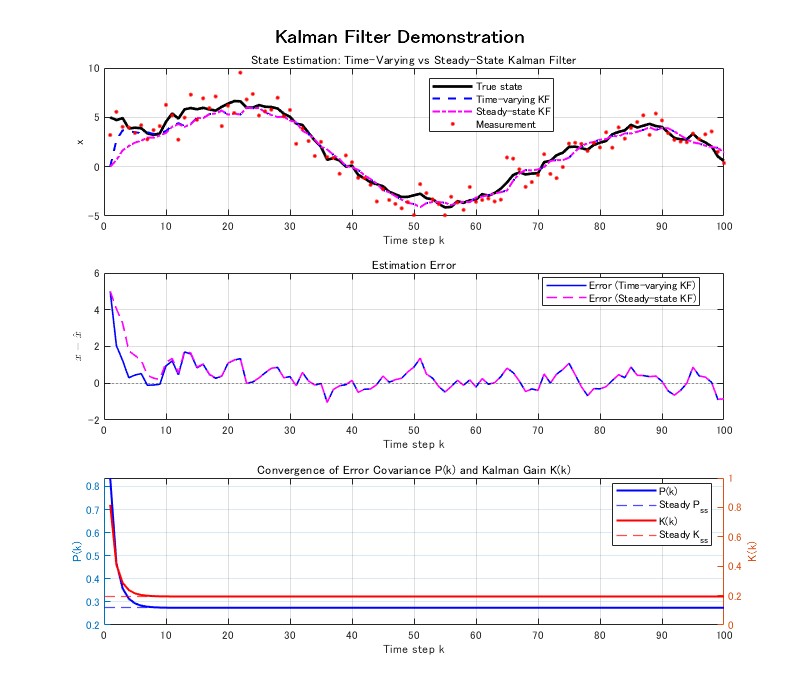
Steady-State Kalman Filter: Comparison of True State, Measurement, and Estimate

The MATLAB code for generating this figure is available at: MATLAB_state_observer/03_kalman_filter

Duality with LQR

There is a fundamental duality between the Kalman filter and the Linear Quadratic Regulator (LQR):

The LQR minimizes a quadratic cost on the state and input for a deterministic system, leading to a state feedback gain via the Riccati equation.
The Kalman filter minimizes the estimation error covariance for a stochastic system, leading to an observer gain via the dual Riccati equation.

This duality means that computational tools developed for LQR (e.g., MATLAB's dlqr function) can also be used to solve the Kalman filter problem, and vice versa.

Continuous-Time Kalman-Bucy Filter

For continuous-time systems:

$\displaystyle \dot{x}(t) = Ax(t) + Bu(t) + B_d w(t)$

$\displaystyle y(t) = Cx(t) + v(t)$

where $w(t)$ and $v(t)$ are continuous-time white noise processes with intensities $Q$ and $R$ , the Kalman-Bucy filter is given by:

$\displaystyle \dot{\hat{x}}(t) = A\hat{x}(t) + Bu(t) + K_f(t)\bigl(y(t) - C\hat{x}(t)\bigr)$

$\displaystyle K_f(t) = P(t)C^T R^{-1}$

where the error covariance $P(t)$ satisfies the continuous-time Riccati equation:

$\displaystyle \dot{P}(t) = AP(t) + P(t)A^T - P(t)C^T R^{-1} CP(t) + B_d Q B_d^T$

The steady-state version is obtained by setting $\dot{P} = 0$ and solving the resulting continuous algebraic Riccati equation (CARE), which can be computed using MATLAB's care function.

For the relationship between continuous-time and discrete-time formulations, see: Discretization of Continuous-Time Control Systems

Tuning the Kalman Filter: Choosing Q and R

In practice, the noise covariances $Q$ and $R$ are often not known precisely. The tuning of $Q$ and $R$ is therefore a critical practical issue:

Measurement noise covariance $R$ can often be estimated from sensor specifications or by analyzing sensor data when the system is at rest.
Process noise covariance $Q$ is more difficult to determine. It represents the model uncertainty and is typically tuned based on engineering judgment or experimental validation.
A common approach is to start with $Q = q I$ and $R = r I$ with scalar tuning parameters $q$ and $r$ , and adjust their ratio $q/r$ to achieve the desired estimation performance.
Increasing $q/r$ makes the filter more responsive (faster tracking) but more sensitive to measurement noise.
Decreasing $q/r$ makes the filter smoother but slower to respond to state changes.

When the noise statistics are poorly known, the H-infinity filter provides an alternative that guarantees worst-case performance without relying on Gaussian noise assumptions.

For the H infinity filter approach using LMI optimization, see: H infinity Filter: Robust State Estimation Using LMI Optimization

Extensions of the Kalman Filter

Extended Kalman Filter (EKF)

For nonlinear systems of the form:

$\displaystyle x(k+1) = f\bigl(x(k), u(k)\bigr) + B_d w(k)$

$\displaystyle y(k) = h\bigl(x(k)\bigr) + v(k)$

the Extended Kalman Filter (EKF) linearizes the system around the current state estimate at each time step and applies the standard Kalman filter equations to the linearized system. The Jacobian matrices $F(k) = \partial f / \partial x$ and $H(k) = \partial h / \partial x$ replace $A$ and $C$ in the prediction and update equations.

The EKF is the most widely used nonlinear state estimator in practice, particularly in navigation (GPS/INS) and robotics (SLAM). However, it is not guaranteed to be optimal for nonlinear systems, and may diverge if the initial estimate is far from the true state or if the nonlinearity is strong.

Unscented Kalman Filter (UKF)

The Unscented Kalman Filter (UKF) uses a set of deterministically chosen sigma points to capture the mean and covariance of the state distribution as it propagates through the nonlinear system. Unlike the EKF, the UKF does not require Jacobian computation and generally provides better accuracy for highly nonlinear systems.

Multi-Rate Kalman Filter

In many practical systems, sensors operate at different sampling rates. For example, in automotive applications, GPS may update at 1–10 Hz while wheel speed sensors operate at 100 Hz. The standard Kalman filter assumes all measurements arrive at a uniform rate and does not directly handle this situation.

The multi-rate Kalman filter addresses this by modeling the multi-rate system as a periodically time-varying system where the observation structure changes cyclically depending on which sensors are active at each time step. The Kalman gains converge to periodic steady-state values that repeat every frame period $M$ (the least common multiple of all sensor periods).

A key challenge in the multi-rate setting is that the cyclic reformulation used to convert the periodically time-varying system into an LTI system produces a measurement noise covariance matrix $\check{R}$ that is only positive semidefinite (not positive definite), because at certain time instants some sensors are inactive and contribute zero rows. This prevents direct application of the standard Riccati equation.

This challenge is addressed by an LMI optimization approach based on the dual LQR formulation, which naturally handles semidefinite covariance matrices. The LMI framework also enables multi-objective design, including:

Pole placement constraints for guaranteed convergence rates
Mixed H₂/l₂-induced norm design for balancing average-case and worst-case estimation performance

For the detailed LMI-based multi-rate Kalman filter design method, see the paper: H. Okajima, LMI Optimization Based Multirate Steady-State Kalman Filter Design, arXiv:2602.01537 (2026, submitted).

For the multi-rate observer design using l₂-induced norm, see: State Observer Under Multi-Rate Sensing Environment and Its Design Using l2-Induced Norm

Relationship Between Kalman Filter and Luenberger Observer

The following table clarifies the relationship between the Kalman filter and the basic Luenberger observer.

Aspect	Luenberger Observer	Kalman Filter
System model	Deterministic	Stochastic (with noise)
Gain design	Manual (pole placement, LMI)	Automatic (minimizes error covariance)
Optimality	No optimality guarantee	Optimal for Gaussian noise
Requires noise statistics	No	Yes (Q, R)
Steady-state form	Time-invariant observer	Time-invariant (steady-state KF)
Mathematical structure	Same — both are feedback estimators with gain L or K

In the steady-state case, the Kalman filter is a Luenberger observer with a specific, optimally computed gain. This means that all the theoretical properties of the Luenberger observer (stability via eigenvalue placement, separation principle, etc.) also apply to the steady-state Kalman filter.

Multi-Rate State Observer — H. Okajima, Y. Hosoe and T. Hagiwara, State Observer Under Multi-Rate Sensing Environment and Its Design Using l2-Induced Norm, IEEE Access (2023). Designs a periodically time-varying state observer for multi-rate sensing environments. The LMI-based approach in this paper serves as the foundation for the multi-rate Kalman filter extension.

Multi-Rate Observer-Based Feedback Control — H. Okajima, K. Arinaga and A. Hayashida, Design of observer-based feedback controller for multi-rate systems with various sampling periods using cyclic reformulation, IEEE Access (2023). Extends the multi-rate observer to a complete feedback control system.

Multi-Rate System Identification — H. Okajima, R. Furukawa and N. Matsunaga, System Identification Under Multirate Sensing Environments, Journal of Robotics and Mechatronics, Vol. 37, No. 5, pp. 1102–1112 (2025). Provides the system identification algorithm that obtains the plant model required for Kalman filter design in multi-rate environments.

Outlier-Robust State Estimation (MCV Observer) — When sensor measurements contain outliers (large sporadic errors), the standard Kalman filter performance degrades significantly. The MCV observer provides a robust alternative using median-based estimation.

Model Error Compensator (MEC) — When there is a gap between the plant model and the actual system, the Model Error Compensator can enhance robustness of the observer-based control system.

MATLAB Code

GitHub (Kalman Filter Simulation): MATLAB_state_observer/03_kalman_filter
GitHub (Multi-Rate Kalman Filter): multirate-kalman-filter
MATLAB File Exchange (Multi-Rate Observer): State Estimation under Multi-Rate Sensing: IEEE ACCESS 2023
GitHub (LMI basics): MATLAB Fundamental Control LMI

Paper Information

Okajima, "LMI Optimization Based Multirate Steady-State Kalman Filter Design", arXiv preprint, arXiv:2602.01537 (2026, submitted).

Self-Introduction

Hiroshi Okajima — Associate Professor, Graduate School of Science and Technology, Kumamoto University. Member of SICE, ISCIE, and IEEE.

www.control-theory.com / Blog / YouTube / GitHub

If you found this article helpful, please consider bookmarking or sharing it.

KalmanFilter #StateEstimation #StateObserver #LMI #MultiRateSystems #SensorFusion #DiscreteTimeControl #ControlEngineering #Riccati #MATLAB

制御工学ブログ

Kalman Filter: From Basic Algorithm to Multi-Rate Extensions

Why the Kalman Filter Matters