モデル誤差抑制補償器のPythonによる無料制御シミュレーション

この記事では、モデル誤差抑制補償器（Model Error Compensator）のPython（Google colaboratory）を用いた無料制御シミュレーションについての説明をします。

まず、制御シミュレーションに必要なPythonライブラリをインストールします。すべて無料で利用できます。

各ライブラリの役割：

control: 制御システムの解析・設計専用ライブラリ
numpy: 数値計算の基盤
matplotlib: グラフ描画・可視化

Google colaboratoryのコードは以下でシェアします。自身の環境にコピーし、上から順番にコードのセルを実行していってください。上記のライブラリインストールもコード内に含んでいますのでGoogleアカウントがあればすぐに実行できます。

colab.research.google.com

以下は，上記のコードを実行した際の各種グラフです。MECの概要については以下のぺージを確認ください。

blog.control-theory.com

制御対象は以下のように設定しています。

\begin{eqnarray} P = \frac{K}{Ts+1}\frac{1}{s+2} \end{eqnarray}

このとき， $T$ と $K$ は±10%の誤差を含みます。

一方，MECにより補償された制御対象は以下のように応答のバラツキが抑えられます。

MECは，制御器を含む制御系に適用するため，閉ループ系の応答も示します。

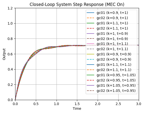
MECを適用することにより，閉ループ応答のばらつきも抑えられ，定常偏差も残っていないことが確認できます。誤差をより小さくしたい場合は，誤差補償器のパラメータを変えればよいです。

コードは以下の通りです。

Installation

!pip install control numpy matplotlib

Python Code

import numpy as np
import matplotlib.pyplot as plt
import control.matlab as control_matlab

# Based on the MATLAB code (assuming the transfer functions are defined within the script)
# Let's assume the MATLAB code has something like:
# % Mechanical system transfer function (e.g., from motor voltage to load speed)
# pm_num = [1];
# pm_den = [0.1, 1]; # Example: 0.1s + 1
# pm = tf(pm_num, pm_den);

# % Disturbance transfer function (e.g., from disturbance torque to load speed)
# d_num = [0.5];
# d_den = [0.1, 1]; # Example: 0.5 / (0.1s + 1)
# d = tf(d_num, d_den);

# % Controller transfer function (e.g., a simple proportional controller)
# c_num = [10]; # Example: Kp = 10
# c_den = [1];
# c = tf(c_num, c_den);

# Define the transfer function pm based on the MATLAB code
# pm = tf([1],[1 3 2]);
pm_num = [1]
pm_den = [1, 3, 2]
pm = control_matlab.tf(pm_num, pm_den)

# Define the transfer function d based on the MATLAB code (High Gain)
# d = tf([300 100],[1 0]);
d_num = [300, 100]
d_den = [1, 0]
d = control_matlab.tf(d_num, d_den)

# Define the transfer function c based on the MATLAB code
# c = tf([3 5],[1]);
c_num = [3, 5]
c_den = [1]
c = control_matlab.tf(c_num, c_den)

# Print the defined transfer functions
print("Transfer function pm:")
print(pm)

print("\nTransfer function d:")
print(d)

print("\nTransfer function c:")
print(c)

# k = [0.9,1.1,1,1,0.9,1.1,0.95,1.05];
# t = [1,1,0.9,1.1,0.9,1.1,1.05,0.95];
ks = [0.9, 1.1, 1, 1, 0.9, 1.1, 0.95, 1.05]
ts = [1, 1, 0.9, 1.1, 0.9, 1.1, 1.05, 0.95]

time_vector = np.linspace(0, 10, 500) # Define a suitable time vector for step response

# Create separate figures for MEC on and MEC off open-loop responses
plt.figure() # Figure for Open-loop, MEC on
plt.title('Open-Loop System Step Response (MEC On)')
plt.xlabel('Time')
plt.ylabel('Output')
plt.grid(True)

plt.figure() # Figure for Open-loop, MEC off
plt.title('Open-Loop System Step Response (MEC Off)')
plt.xlabel('Time')
plt.ylabel('Output')
plt.grid(True)

# for k in ks:
#     for t in ts:
for i in range(len(ks)): # Iterate using index to access corresponding k and t
    k = ks[i]
    t = ts[i]
    # Calculate the plant transfer function p
    # p = tf([k(i)],[t(i) 1])*tf([1],[1 2]);
    p = control_matlab.tf([k], [t, 1]) * control_matlab.tf([1], [1, 2])

    # Calculate the compensated plant pc using the MEC formula
    # pc = p*(1+pm*d)/(1+p*d);
    pc = p * (1 + pm * d) / (1 + p * d)

    # Calculate step response for pc (MEC On)
    yout_pc, T_pc = control_matlab.step(pc, time_vector)
    plt.figure(1) # Select the first figure (MEC On)
    plt.plot(T_pc, yout_pc, label=f'pc (k={k}, t={t})') # Plot on the same figure

    # Calculate step response for p (MEC Off)
    yout_p, T_p = control_matlab.step(p, time_vector)
    plt.figure(2) # Select the second figure (MEC Off)
    plt.plot(T_p, yout_p, linestyle='-', label=f'p (k={k}, t={t})') # Plot on the same figure

# Add legends and save figures after the loop
plt.figure(1)
plt.legend()
plt.savefig("open_loop_mec_on_step_responses.png")

plt.figure(2)
plt.legend()
plt.savefig("open_loop_mec_off_step_responses.png")

plt.show()
plt.close('all') # Close all figures