State Feedback Control: Design Gains using Optimal Regulators

This article explains controller design based on optimal regulators for linear systems represented by state equations. Optimal regulators are a type of optimal control, also known as LQ control or LQR (Linear Quadratic Regulator). For an overview including state feedback control models expressed as state equations, refer to the following article.

Summary of State Feedback Control and Control Based on State Equations

State Feedback Control Structure of Optimal Regulators
Concept of Optimal Regulator
Solution to the Optimal Regulator Problem
Verification of Optimal Regulator Using Numerical Example

State Feedback Control Structure of Optimal Regulators

Now, let’s explain state feedback, optimal control, and optimal regulators. Optimal regulators are one of the basic design methods widely known in the field of control engineering.

First, an explanation of state feedback. The control object expressed as a state equation is given as follows:

State Equation

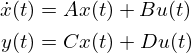
The control input is u, and the control output is y. In many cases, D=0. The state is x. In state feedback,

the input is used by multiplying the state by a coefficient. Here, symbols such as K and F are used as examples, but the symbols used vary depending on the paper. In some cases, a minus sign is explicitly attached before the symbol. Examples of state quantities of a control object include speed and position, but for more details, refer to the explanation of the state equation.

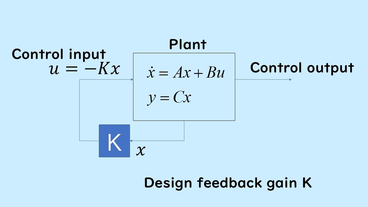
Here, we explain the optimal regulator as a method for determining state feedback gain.

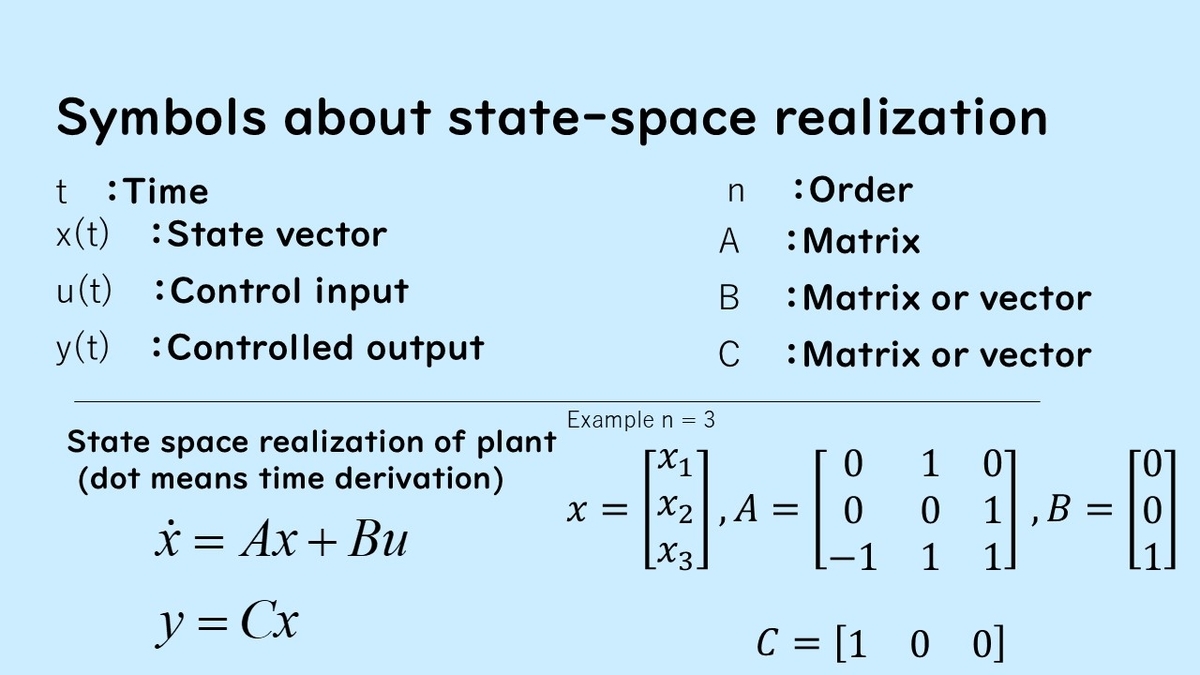
The main symbols in the state equation are as follows. First, t is time, x is the state vector, $u$ is the input, and $y$ is the output. $n$ is the order and corresponds to the number of elements in the state vector. $A$ is an $n$ x $n$ square matrix, $B$ is an $n$ x 1 column vector, and C is a $1 x n$ row vector. However, this is the case where the number of inputs and outputs is one, as shown in the figure.

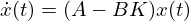
The control law given as follows

is applied to give the control system (autonomous system) as follows.

Concept of Optimal Regulator

Next, we explain what is considered in the optimal regulator problem.

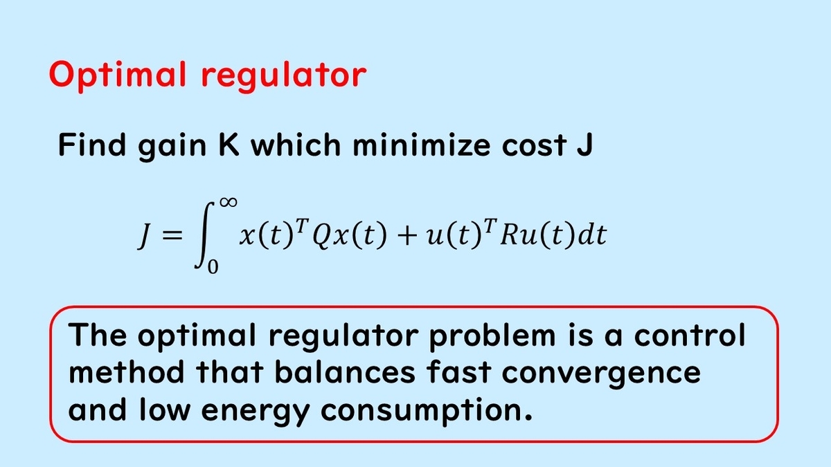
Optimal regulator problem (Cost and Weight)

In the optimal regulator problem, the following evaluation function is considered.

This evaluation function is a quadratic form applied to the state x with Q and expressed as a linear sum with a quadratic form term concerning Ru. The evaluation interval is from time t = 0 to infinity. The reason it is called LQR is from the initials of (Linear Quadratic).

The problem of finding a gain K that minimizes this evaluation function value J is called the optimal regulator problem. Here, the evaluation interval is taken from time 0 seconds to infinity for convenience, but it can start from another time.

The coefficient matrices Q and R of this quadratic form are called weighting matrices. Q is taken large if emphasis is placed on x, and R is taken large if emphasis is placed on the input u. The smaller the first term, the better the solution, which means that x converges to zero quickly. On the other hand, the smaller the second term, the better the solution, which means that less input energy is required.

The optimal regulator problem can be said to be a control method that balances fast convergence and low energy.

Solution to the Optimal Regulator Problem

Here, the solution to the optimal regulator problem is explained first. The solution to the optimal regulator problem has already been obtained and can be found through the following steps.

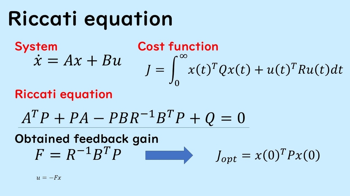
Solving step of optimal regulator problem using riccati equation

First, as shown in step 1 of the figure, find the positive definite matrix P that satisfies this equation called the Riccati equation (Liccati equation). This is the first step.

This solution can be obtained as algebraic computation.

Then, in step 2, using the obtained solution P, the gain is set by multiplying the inverse matrix of R by the transpose of B and by P, which becomes the optimal solution to the previous optimal regulator problem.

For proof of optimality, refer to the video in the latter part.

Verification of Optimal Regulator Using Numerical Example

When finding the gain K in MATLAB, you can use the lqr function to solve the Riccati equation and find the gain K.

Here, consider the design example of an optimal regulator for a system of order n = 3.

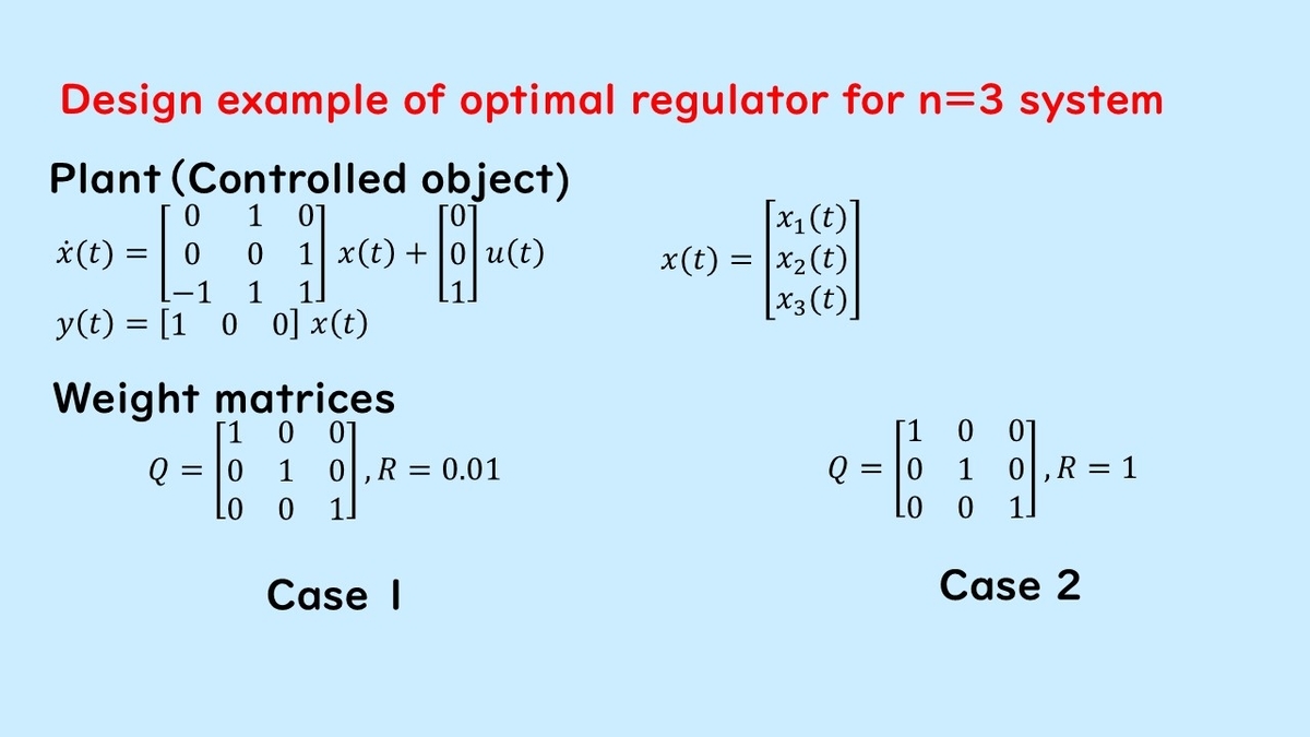
The control object is given as such, with the state vector having three elements. Initially, simulate the case where the elements of the weight matrix are given as the identity matrix and the weight of R is 0.01.

Subsequently, simulate the case where the evaluation value, which aims for more energy savings, focuses on the input. R = 1 and R = 100 are shown.

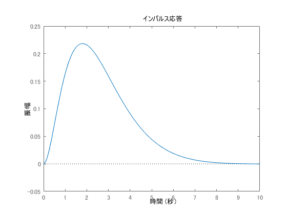
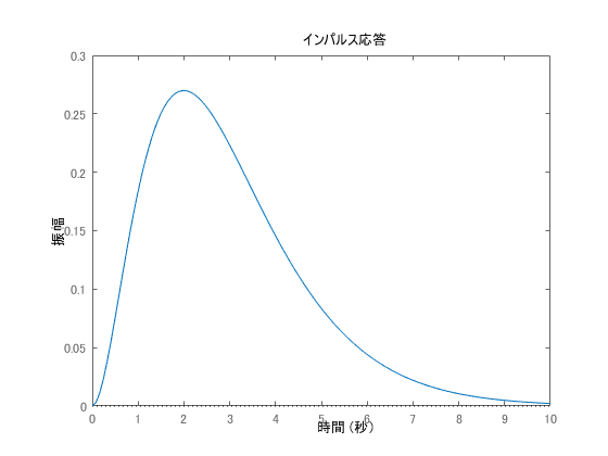
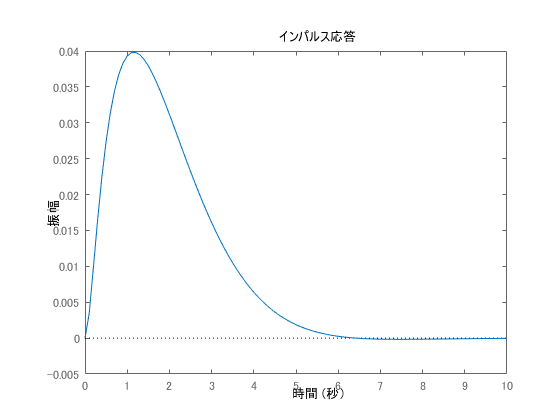
It can be seen that the larger the R, the more the control results allow larger amplitudes. The waveform is not shown for the input, but when showing the time transition of $u = K x$ , $u$ becomes a smaller value (time series) as the weight of $R$ becomes larger.