This article summarizes the equivalent transformation (coordinate transformation, equivalence transformation) of a system expressed by a state equation. A video explaining the equivalent transformation of state equations is provided at the bottom.
The overall picture of state feedback control is summarized in the following article.
Summary of State Feedback Control and Control Based on State Equations
- Representation of State Equations
- Steps for Equivalent Transformation of State Equations
- Properties Preserved Before and After Equivalent Transformation
- Video on Equivalent Transformation of State Equations
Representation of State Equations
First, consider a system where the dynamics of the control object are given as a state equation representation, as shown in the following figure. Control based on state equations is one of the fundamental topics in control engineering.
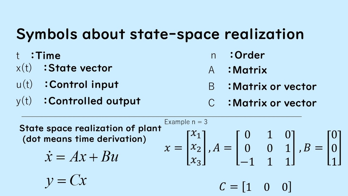
The control input is u, the control output is y, and the state is x. The order of the control object is n, and the number of elements in the state vector is n.
Moreover, A, B, and C are square matrices of order n, and B is a column vector of order n for single-input cases. If there are multiple inputs, B takes the form of a matrix. For single-output cases, C is a row vector of order n.
Overview of Equivalent Transformation (Coordinate Transformation)
In equivalent transformation, we consider transforming the state equation concerning state x into a state equation concerning \tilde x. Equivalent transformation can also be called coordinate transformation or equivalence transformation. Here, we proceed with the explanation as equivalent transformation.
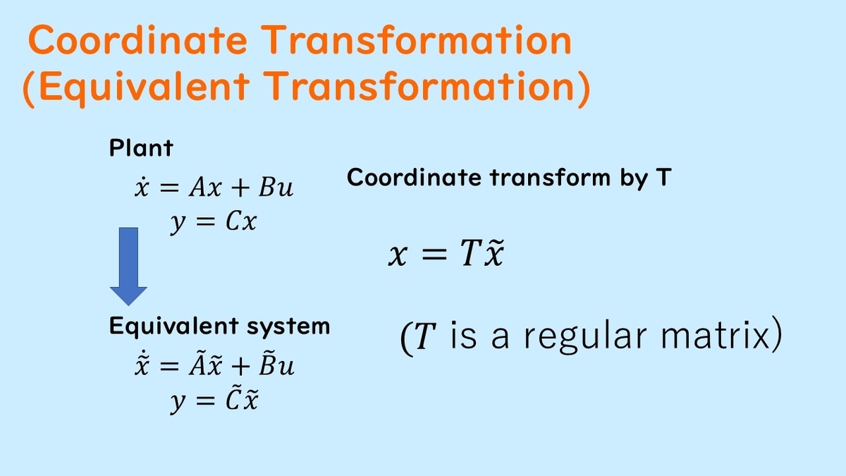
Here, in the figure, matrix T is a regular matrix, meaning it has an inverse matrix. Using matrix T allows us to change the way the state coordinates are taken. This allows us to obtain a state equation concerning a different state \tilde x, satisfying the same input-output characteristics through equivalent transformation.
Steps for Equivalent Transformation of State Equations
Now, let's explain the method of equivalent transformation. The following figure shows the flow of equivalent transformation.
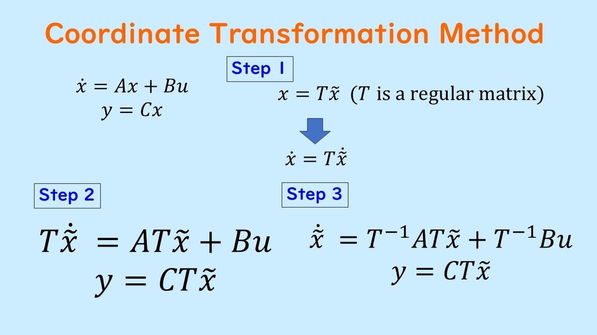
First, when a state equation is given, we set the state transformation as
![]()
. At this time, using the inverse matrix of T, the following also holds:
![]()
Here, differentiating the equation with respect to time on both sides gives
![]()
.
Considering this, we move to the steps.
By substituting the above two equations into the original state equation, we obtain the equation described in Step 1. By multiplying both sides of the equation obtained in Step 1 by the inverse matrix of T from the left, we obtain Step 2, and then
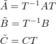
by doing so, the equivalent transformation is completed. Note that if there is a direct current component (direct term), D does not change before and after the transformation.
Properties Preserved Before and After Equivalent Transformation
The following properties are preserved before and after this equivalent transformation:
- The transfer functions derived from each state equation match in both
- The poles of the control object (eigenvalues of matrix A and eigenvalues of matrix \tilde A) completely match
- The properties of controllability and observability match
First, because the transformation preserves the input-output characteristics, the transfer functions converted from both will match.
Second, concerning poles, it is evident from the matching transfer functions that the poles of both systems match, and the eigenvalues of matrix A and matrix \tilde A completely match.
Third, if the system before equivalent transformation is controllable, it remains controllable after equivalent transformation, and if it is uncontrollable before, it remains uncontrollable after, preserving these properties.
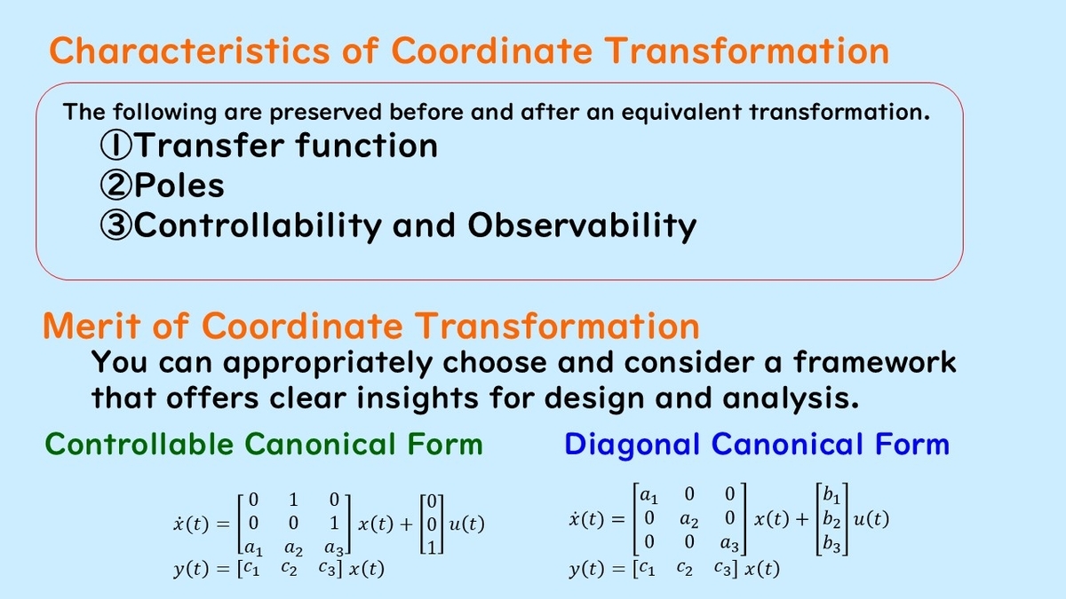
Benefits of Equivalent Transformation
Controllable Canonical Form
Finally, let me conclude by explaining the benefits of equivalent transformation. By performing equivalent transformation, there is the advantage of being able to think in a framework with good prospects for design and analysis. For example, if the original system is controllable, equivalent transformation can convert it to a controllable canonical system. This allows easy implementation of pole placement and other analyses.
Diagonal Canonical Form
Additionally, converting to a diagonal canonical system allows for thorough examination of the relationship between the system modes.
This concludes the explanation of equivalent transformation.
Video on Equivalent Transformation of State Equations
Related Pages (Equivalent Transformations)
Equivarent transformation is a prerequisite for state observer design. For a comprehensive guide, see: State Observer and State Estimation: A Comprehensive Guide
Equivarent transformation is a prerequisite for state feedback design. For a comprehensive guide, see: State Feedback Control and State-Space Design: A Comprehensive Guide