State Feedback Control: Design Gains using Pole Placement

This article summarizes state feedback control for systems expressed in state equation form. It particularly touches on gain design using pole placement methods and the relationship between pole placement and performance. At the end, you can find control simulations and related videos to watch together with this article.

For an overview of state feedback control, see the following article:

Summary of State Feedback Control and Control Based on State Equations

State Equations and Feedback Control
- State Equation Representation of Control Targets
- State Feedback Control and Autonomous Systems
System Poles and Control Performance Arranged by Pole Placement
Pole Placement in Controllable Canonical Form
Related Videos on State Feedback Control
- Pole Placement Using MATLAB Simulation
- Related Pages (Pole Placement)

State Equations and Feedback Control

State Equation Representation of Control Targets

State feedback control is a method (control law) that controls by multiplying state variables by coefficients, as shown in the figure. It is one of the fundamental control system design theories in control engineering.

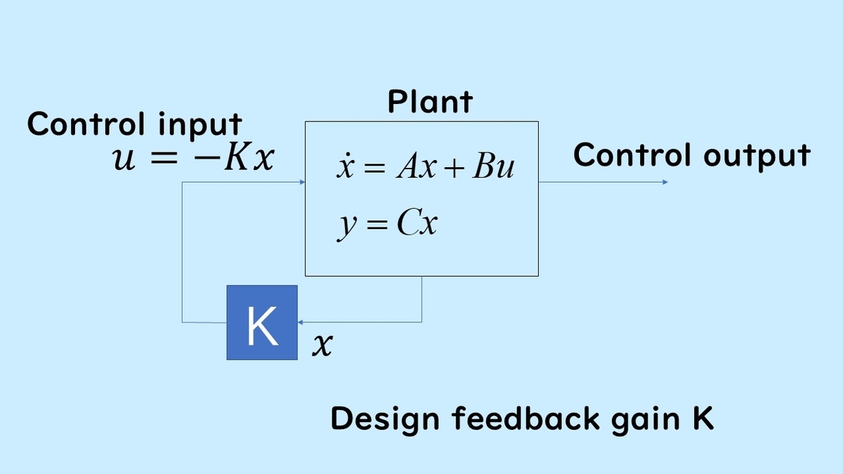
This explains state feedback. When the control target is given in the form of a state equation, the control input is $u$ , and the control output is $y$ . In state feedback, the control input is expressed as $u = - Kx$ , where the input is a product of state variables and coefficients.

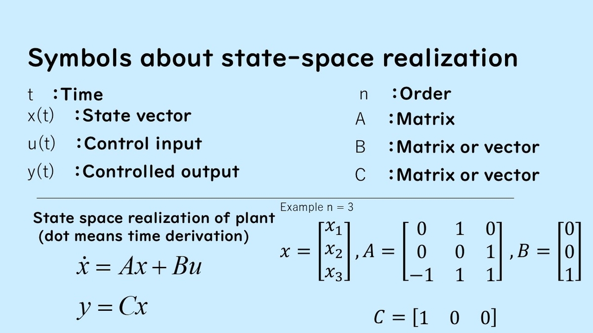
The symbols in the above diagram represent the main elements of the state equation. $t$ represents time, $x$ is the state vector, $u$ is the input, and $y$ is the control output. The order of this system is represented by the symbol $n$ , which is an integer greater than or equal to 1.

For more details on the state equation representation, see here:

blog.control-theory.com

State Feedback Control and Autonomous Systems

By providing the input $u$ as - Kx to the system given as a state equation, the following autonomous system is obtained:

$\dot x(t) = (A-BK)x(t)$

The dynamics of the system with state feedback are determined by the matrix A-BK.

In the control law, there are various ways to express the feedback gain and control law, such as $u = -Kx$ , $u = Kx$ , or $u = Fx$ . Here, we proceed with $u = -Kx$ .

For example, when n = 3, K is in the following vector form:

$K = [k_1\,\, k_2\,\, k_3$ ]

Also, when the number of inputs is 2 for the same n = 3, K is in the following matrix form:

State feedback gain

System Poles and Control Performance Arranged by Pole Placement

Before explaining pole placement, let us first explain poles. The eigenvalues of the matrix A-BK are the poles of the feedback system and are also the roots of the following characteristic equation:

$|sI - (A-BK)| = 0$

When the feedback gain K is determined, the value of the poles varies accordingly.

The roots of the characteristic equation, the poles of the control system, are equal, so (if controllable), the poles of the control system can be freely manipulated.

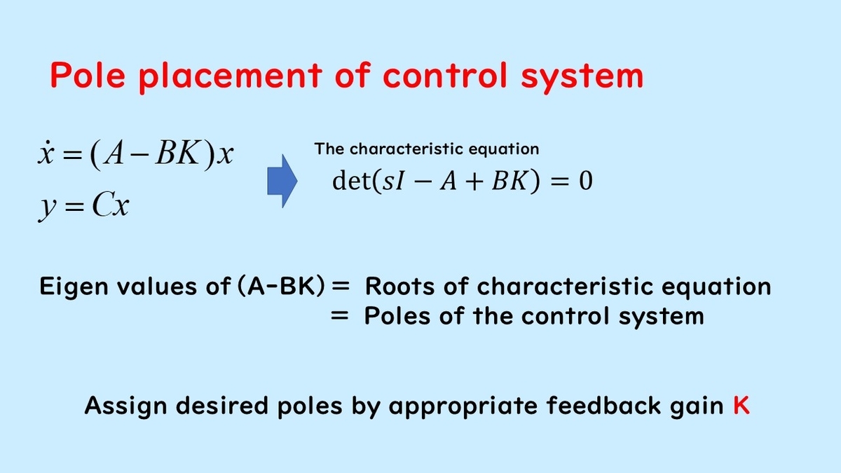
In pole placement, it is important to place the poles of $A-BK$ in appropriate locations by determining the feedback gain $K$ .

The eigenvalues of the matrix are the poles, so there are $n$ poles in total. Also, if all poles are on the left side of the complex plane, the system is asymptotically stable, which is the minimum requirement for setting the gain $K$ .

Poles and Responses of Scalar Systems

In scalar systems ( $n = 1$ ), $A, B, K$ are scalar values. The pole is $A-BK \in R^{1\times 1}$ . The autonomous system is given by:

$\dot x (t) = (A-BK)x(t)$

The solution trajectory is:

$x(t) = exp( (A-BK)t )x(0) = e^{(A-BK)t}x(0)$

If the value of $A-BK$ is negative, the value of $x$ converges to zero as $t$ increases (stable). On the other hand, if it is positive, it diverges (unstable).

Poles and Stability

Similar to scalar systems, even if $n \geq 2$ , the poles asymptotically approach zero if their real parts are negative, and the system diverges if there is even one pole with a positive real part. For the system to be stable, all poles must be on the left side of the complex plane.

Let's look at an example. Here is an example of a 3rd order system with $n = 3$ .

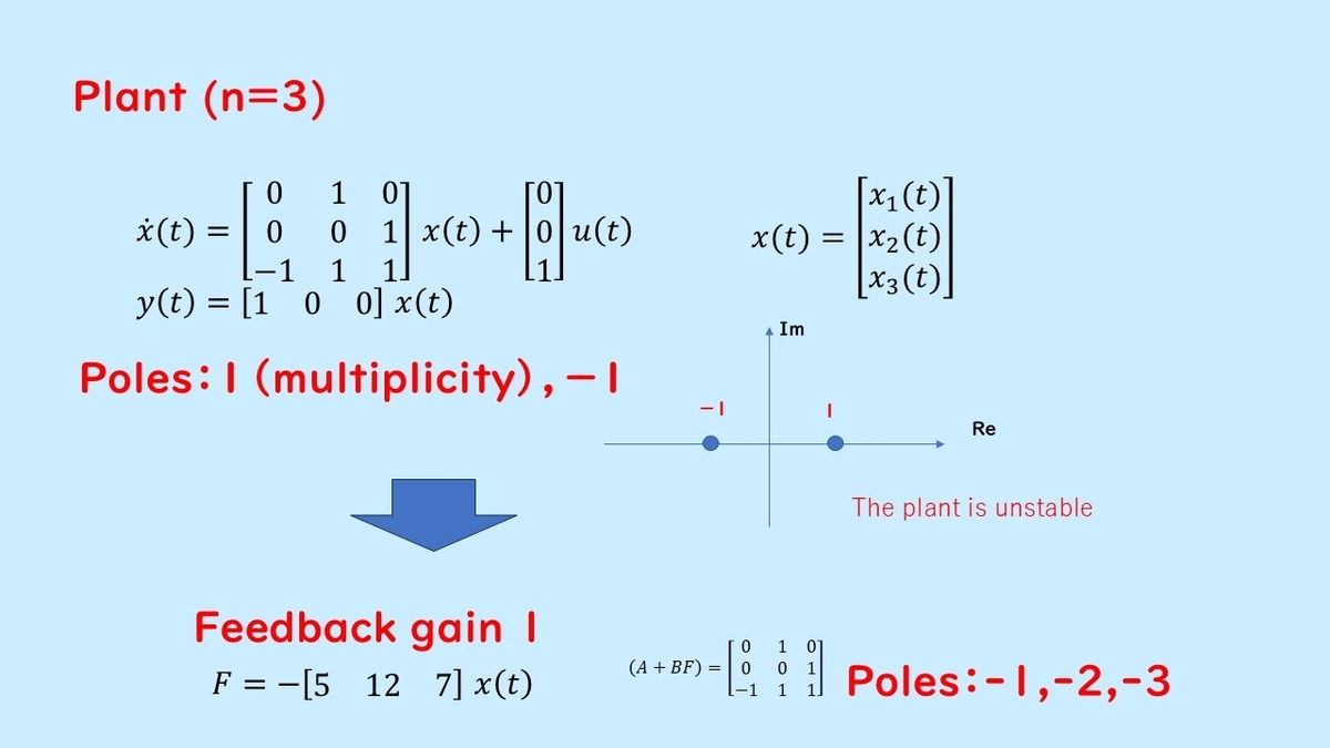
This control target has 3 state variables, and the eigenvalues of the a matrix, which are the poles of the system, are 1 (double root) and -1. Since not all poles are in the left plane, the state of this system diverges if the input $u$ is 0, meaning it is an unstable system.

Next, by giving the state feedback

$K = [5\,\,12\,\, 7$ ]

, the poles can be set to -1, -2, and -3. As a result, even if the original system is unstable, it can be stabilized by pole placement.

Pole Placement and Control Performance

Real Parts of Poles and Response

Next, I will explain the behavioral differences that result from the placement of poles (where the poles are positioned). In the diagram below, Gain 2 has poles positioned closer to the imaginary axis, specifically at -0.5, -1, and -2, still on the left half-plane. Meanwhile, Gain 3 has poles positioned further to the left, at -5, -6, and -7. The feedback gains K for achieving each pole placement are different.

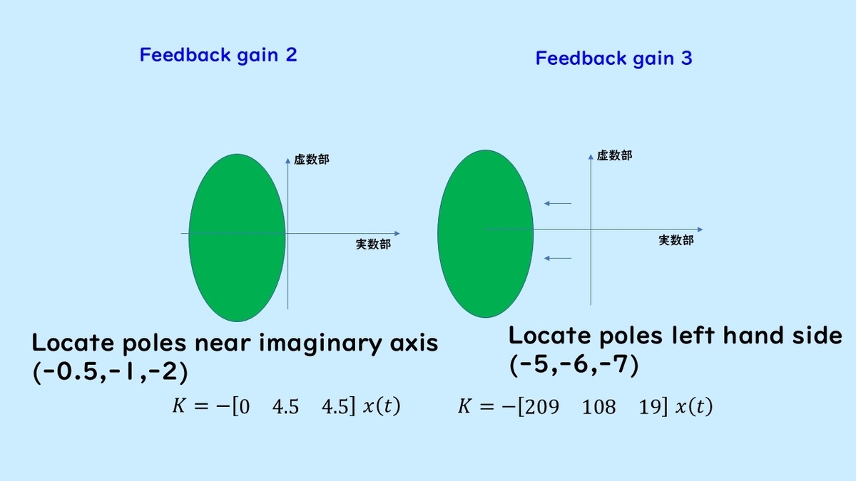
In this case, positioning poles further to the left, as in Gain 3, allows the system to converge to the origin more quickly, resulting in a faster response than Gain 2.

The response waveform obtained by the pole placement method for a system with 3 state variables is shown in blue for $-10, -15\pm 3i$ and in orange for $-4, -3\pm 3i$ .

Numerical simulation of pole placement method — Comparison of Response Waveforms (Comparison of Two Types with Different Real Parts)

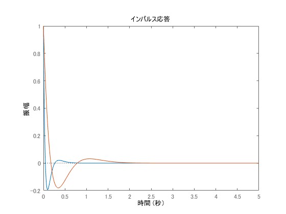
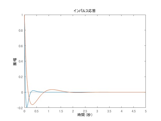
It can be seen that the blue one converges to zero more quickly. Next, a numerical simulation is shown where only part of the poles is changed. The blue one is $-10, -15\pm 3i$ , and the orange one is $-10, -2\pm 3i$ . In this case, it can be confirmed that the response is significantly slower when one of the conjugate poles is positioned closer to zero, as in the orange one.

Numerical simulation of pole placement method 2 (changing some pole placements) — Comparison of Responses (Comparison of Two Types with Some Poles Changed)

Other numerical simulations can also be confirmed from the videos below.

Imaginary Parts of Poles and Response

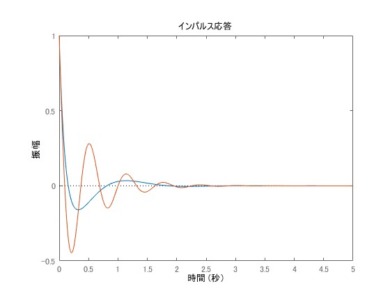
Next, I will compare poles placed far from the real axis in Gain 4 and Gain 5 with poles placed closer to the real axis.

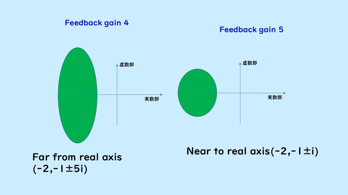
When the poles are placed at -2, -1± 5i, far from the real axis, the response waveform is oscillatory. In contrast, when placed closer to the real axis, there is less oscillation.

Let's look at an example through numerical simulations. The blue one is $-10, -2\pm 3i$ , and the orange one is $-10, -2\pm 10i$ . Here, while changing only the imaginary part values without changing the real parts, it can be seen that the response becomes more oscillatory.

Numerical simulation of pole placement method 3 (changing some pole placements) — Comparison of Pole Placements (Size of Imaginary Parts and Response)

Summary of Poles and Response

First, there are n poles in a system of order n. The system is asymptotically stable if all poles are on the left side of the complex plane.

When placing poles, it is important not to place them too far from the real axis to avoid oscillations. Placing poles not too far from the real axis is essential.
Additionally, positioning the poles further to the left of the imaginary axis to speed up convergence will result in faster convergence.

On the other hand, if placed too far from the imaginary axis, the physical values of the input signal tend to be large, so it is necessary to determine the placement according to the range of input that can be applied to the system.

There are also various constraints, such as ensuring the poles are not too close to each other.

Pole Placement in Controllable Canonical Form

Let's explain pole placement for controllable canonical systems. When the control target is expressed in a state equation form, the problem of finding the state feedback gain K to achieve specified poles is considered. This problem is called the pole placement problem.
Here, the control input u is given in the form of a proportional coefficient to the state as:

$u(t) = -Kx(t)$

This defines the control output. Here, we assume that the control target is controllable. If controllable, it can be transformed into a controllable canonical form.

Control Law and Structure of Controllable Canonical Form

Let's look at the controllable canonical system. First, the structure of a second-order controllable canonical system is as follows:

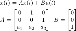
Next, the structure of a third-order system is as follows:

Controllable Canonical Form

For a system given in controllable canonical form, the characteristic equation with the control law u = -Kx is given as follows:

Characteristic Equation for Second Order

$s^2+(a_2 - k_2)s + (a_1 - k_1) = 0$

Characteristic Equation for Third Order

$s^3 + (a_3-k_3)s^2+(a_2-k_2)s+(a_1-k_1) = 0$

In each case, feedback gains can be obtained by determining the coefficients K to make the roots of the characteristic equation ideal. For example, for a second-order control target where the poles (characteristic roots) are set to -2 and -1, the ideal characteristic equation is:

$s^2+3s+2 = (s+2)(s+1) = (s-(-2))(s-(-1))=0$

Feedback gains can be obtained by determining $k_1,k_2$ to match these coefficients. Similarly, if you want to place complex numbers (e.g., -2±i), you can match it to:

$s^2+4s+3=(s+2)^2+1=(s+2-i)(s+2+i)=0$

By setting $k_1,k_2$ to match the coefficients 4 and 3, you can place the poles. Thus, the characteristics of the control system can be determined by pole placement. Note that if the system is not controllable, some poles cannot be placed as desired.

State feedback control can be used when all state variables (elements of the state vector) can be measured. On the other hand, if the number of outputs is less than the number of states, the system is configured as an output feedback control system by incorporating an observer. This concludes the explanation of this article.