This article summarizes partial fraction decomposition. We will explain how to decompose rational functions using partial fraction decomposition and its use in control engineering. Links to videos and related articles that explain partial fraction decomposition are placed at the bottom.
- Overview of Partial Fraction Decomposition
- Example of Simple Partial Fraction Decomposition and Signal Waveform
- Method of Partial Fraction Decomposition
- Videos and Related Articles on Partial Fraction Decomposition
Overview of Partial Fraction Decomposition
In control engineering, inverse Laplace transforms are used to obtain signal waveforms using Laplace transform tables. The Laplace transform of a signal is given as a rational function of , and if the signal is a first-order or second-order polynomial, the waveform can be determined by the inverse Laplace transform using the transform table. For higher-order cases, partial fraction decomposition is applied to the Laplace transform of the signal given as a rational function, decomposing it into first-order or second-order terms, allowing each term to be inversely transformed to obtain the signal waveform (as a function of time).
Example of Simple Partial Fraction Decomposition and Signal Waveform
Here, a simple example is shown. For a control plant (transfer function representation) , when a unit step input (Laplace transform)
is applied, the control output is given by the following equation.
\begin{equation} y(s) = P(s) r(s) = \frac{1}{(s+2)s} \end{equation}
At this point, can be decomposed into the following form.
\begin{equation} \frac{A}{s+2}+\frac{B}{s}\end{equation}
Here, setting and
satisfies the following equality.
\begin{equation} \frac{1}{(s+2)s}=-\frac{1}{2}\frac{1}{s+2}+\frac{1}{2}\frac{1}{s}\end{equation}
When you want to find , you can derive it by taking the inverse Laplace transform of each term based on the equation above.
\begin{equation} y(t) = -\frac{1}{2} e^{-2t} + \frac{1}{2}\end{equation}
Here, we are dealing with a case where the order of the denominator polynomial is 2, but for higher-order cases, decomposing into lower-order terms can provide a clearer view of the results.
Method of Partial Fraction Decomposition
A rational function is given in the following form.
\begin{equation} Q(s) = \frac{N(s)}{D(s)}\end{equation}
Here, are polynomials of
. In partial fraction decomposition,
is decomposed into a sum of simpler partial fractions. The procedure is as follows.
- Factorization of the Denominator
First, factorize . For example, it can be decomposed into the following form.
\begin{equation} D(s) = (s+a_1) (s+a_2) (s^2 + a_3 s+ b_3) (s+a_4)^2\end{equation}
- Form After Partial Fraction Decomposition
As a result of factorizing the denominator, it is decomposed into the following form.
\begin{equation} Q(s) = \frac{A}{s+a_1} + \frac{B}{s+a_2} + \frac{Cs+D}{s^2+a_3s+b_3}\\ + \frac{E}{s+a_4}+\frac{F}{(s+a_4)^2}\end{equation}
If are found correctly, the equality holds.
- Finding the Coefficients
Basically, you can multiply both sides by the same denominator, compare the coefficients of the numerators to form equations, and solve these simultaneous equations to find .
For first-order factors, the coefficients can be found using the following method. Here, we find the coefficient .
- Multiply
by
.
- The value obtained in step 1,
, with
, becomes
.
In practice, when you multiply by
, the right side of the decomposed expression becomes
, and the other terms become a first-order polynomial of
. Thus, substituting
will zero out all terms except
on the right side.
Response Calculation Using Partial Fraction Decomposition
The step response of a control plant is derived using partial fraction decomposition. The control plant is given by
\begin{equation} P(s) = \frac{s+3}{s^2+3s+2}\end{equation}
and is applied.
At this point, can be described as follows.
\begin{equation}y(s)=\frac{s+3}{s^3+3s^2+2s}\end{equation}
Here, by factorizing, we obtain the following form.
\begin{equation} y(s) = \frac{A}{s+1}+\frac{B}{s+2} + \frac{C}{s}\end{equation}
Here, are obtained as follows.
\begin{equation} A = \lim_{s\rightarrow -1}(s+1)\frac{s+3}{s^3+3s^2+2s}\\=\lim_{s\rightarrow -1}\frac{s+3}{s^2+2s}=-2\end{equation}
\begin{equation} B = \lim_{s\rightarrow -2}(s+2)\frac{s+3}{s^3+3s^2+2s}\\=\lim_{s\rightarrow -2}\frac{s+3}{s^2+s}=\frac{1}{2}\end{equation}
\begin{equation} C = \lim_{s\rightarrow 0}s\frac{s+3}{s^3+3s^2+2s}\\=\lim_{s\rightarrow 0}\frac{s+3}{s^2+3s+2}=\frac{3}{2}\end{equation}
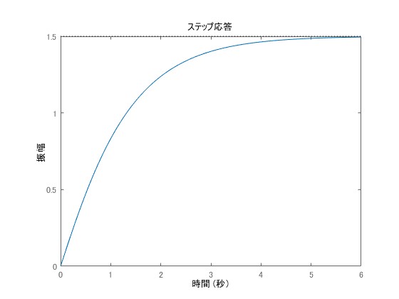
As a result, the output is obtained as follows.
\begin{equation}y(t) = 2e^{-t}-\frac{1}{2}e^{-2t}+\frac{3}{2}\end{equation}
It matches the output waveform below.
Derivation of Diagonal Canonical Form Using Partial Fraction Decomposition
Next, we perform the conversion to state-space representation of a system using partial fraction decomposition. Assume the target is given by
\begin{equation} P(s) = \frac{s+3}{s^2+3s+2}\end{equation}
In this case, can be decomposed into
\begin{equation} P(s) = \frac{A}{s+1}+\frac{B}{s+2}\end{equation}
and are obtained as follows.
\begin{equation} A = \lim_{s\rightarrow -1}(s+1)\frac{s+3}{s^2+3s+2}\\=\lim_{s\rightarrow -1}\frac{s+3}{s+2}=2\end{equation}
\begin{equation} B = \lim_{s\rightarrow -2}(s+2)\frac{s+3}{s^2+3s+2}\\=\lim_{s\rightarrow -2}\frac{s+3}{s+1}=-1\end{equation}
As a result, can be described as follows.
\begin{equation} P(s) = \frac{2}{s+1}-\frac{1}{s+2}\end{equation}
Using independent states to describe it in diagonal canonical form, the state equation of the control plant can be expressed as follows.
\begin{equation} \dot x (t) = A x(t) + B u(t) \\ y(t) = Cx(t)\end{equation}
Where are given as
\begin{equation}A = \begin{bmatrix} -1 & 0\\0 &-2\end{bmatrix}, B = \begin{bmatrix} 1 \\1\end{bmatrix}, C = \begin{bmatrix} 2 & -1\end{bmatrix}\end{equation}
.
Videos and Related Articles on Partial Fraction Decomposition
The following is a video explaining partial fraction decomposition.
Related Articles